Let's talk about MySQL high availability (HA) and synchronous replication once more.
It's part of a longer series on some high availability reference architecture solutions over geographically distributed areas.
Part 1: Reference Architecture(s) for High Availability Solutions in Geographic Distributed Scenarios: Why Should I Care?
Part 2: MySQL High Availability On-Premises: A Geographically Distributed Scenario

The Problem

A question I often get from customers is: How do I achieve high availability in case if I need to spread my data in different, distant locations? Can I use Percona XtraDB Cluster? Percona XtraDB Cluster (PXC), mariadb-cluster or MySQL-Galera are very stable and well-known solutions to improve MySQL high availability using an approach based on multi-master data-centric synchronous data replication model. Which means that each data-node composing the cluster MUST see the same data, at a given moment in time. Information/transactions must be stored and visible synchronously on all the nodes at a given time. This is defined as a tightly coupled database cluster. This level of consistency comes with a price, which is that nodes must physically reside close to each other and cannot be geographically diverse. This is by design (in all synchronous replication mechanisms). This also has to be clarified over and over throughout the years. Despite that we still see installations that span across geographic locations, including AWS Regions. We still see some solutions breaking the golden rule of proximity, and trying to break the rules of physics as well. The problem/mistake is not different for solutions based on-premises or in the cloud (for whatever cloud provider). Recently I had to design a couple of customer solutions based on remote geographic locations. In both cases, the customer was misled by an incorrect understanding of how the synchronous solution works, and from a lack of understanding of the network layer. I decided I need to cover this topic again, as I have done previously in Galera geographic replication and Effective way to check network connection in a geographically distributed environment

What Happen When I Put Things on the Network?

Well, let's start with the basics. While light travels at 300 million meters per second, the propagation of the electric fields or electric signaling is slower than that. The real speed depends by the medium used to transmit it. But it can be said that the real speed normally spans from 0% to 99% of light-speed (depending on the transmission medium). This means that in optimal conditions the signal travels at approximately 299.72Km per millisecond, in good/mid condition about half that at 149.86Km per millisecond, and in bad conditions it could be 3Km per millisecond or less. To help you understand, the distance between Rome (Italy) and Mountain View (California) is about 10,062Km. At light-speed it will take 33.54ms. In good conditions (90% of light-speed) the signal will take 37.26ms to reach Mountain View, and in less optimal conditions it can easily double to 74.53 ms. Keep in mind this is the electric field propagation speed: optimal conditions with no interruption, re-routing and so on. Reality will bring all the kind of interruptions, repeaters and routing. All the physics above works as a baseline. On top of this, each human construct adds functionalities, flexibility and (unfortunately) overhead – leading to longer times and slower speeds. The final speed will be different than the simple propagation of the electric fields. It will include the transmission time of complex signaling using ICMP protocol, or even higher delays with the use of a very complex protocol like TCP/IP, which includes handshaking, package rerouting, re-sending and so on. On top of that, when sending things over the internet, we need to realize that it is very improbable we will be the only user sending data over that physical channel. As such, whatever we have “on the road” will need to face bandwidth limitation, traffic congestion and so on. I had described the difference between protocols (ICMP – TCP/IP) here, clarifying how the TCP/IP scenario is very different from using different protocols like ICMP, or the theoretical approach. What it all means is that we cannot trust the theoretical performance. We must move to a more empirical approach. But we must understand the right empirical approach or we will be misled.

An Example

I recently worked on a case where a customer had two data centers (DC) at a distance of approximately 400Km, connected with “fiber channel”. Server1 and Server2 were hosted in the same DC, while Server3 was in the secondary DC. Their ping, with default dimension, to Server3 was ~3ms. Not bad at all, right? We decided to perform some serious tests, running multiple sets of tests with netperf for many days collecting data. We also used the data to perform additional fine tuning on the TCP/IP layer AND at the network provider. The results produced a common (for me) scenario (not so common for them):

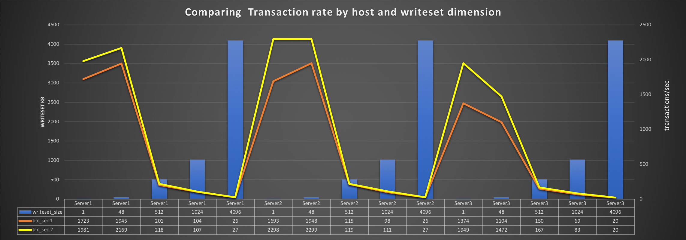
The red line is the first set of tests BEFORE we optimized. The yellow line is the results after we optimized. The above graph reports the number of transactions/sec (AVG) we could run against the different dimension of the dataset and changing the destination server. The full roundtrip was calculated. It is interesting to note that while the absolute numbers were better in the second (yellow) tests, this was true only for a limited dataset dimension. The larger the dataset, the higher the impact. This makes sense if you understand how the TCP/IP stack works (the article I mentioned above explains it). But what surprised them were the numbers. Keeping aside the extreme cases and focusing instead on the intermediate case, we saw that shifting from a 48k dataset dimension to 512K hugely dropped the performance. The drop for executed transactions was from 2299 to 219 on Server2 (same dc) and from 1472 to 167 Server3 (different DC). Also, note that Server3 only managed ~35% fewer transactions comparing to Server2 from the start given the latency. Latency moved from a more than decent 2.61ms to 27.39ms for Server2 and 4.27ms to 37.25ms for Server3.

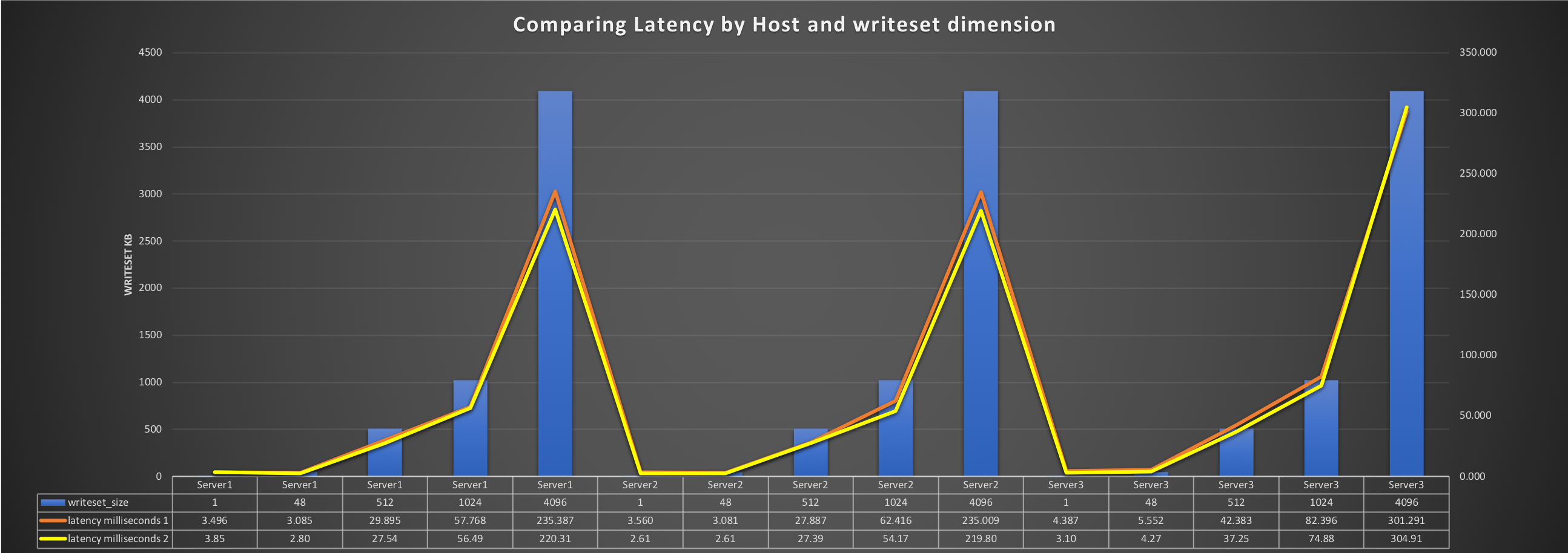
37ms latency is not very high. If that had been the top limit, it would have worked. But it was not. In the presence of the optimized channel, with fiber and so on, when the tests were hitting heavy traffic, the congestion was such to compromise the data transmitted. It hit a latency >200ms for Server3. Note those were spikes, but if you are in the presence of a tightly coupled database cluster, those events can become failures in applying the data and can create a lot of instability. Let me recap a second the situation for Server3: We had two datacenters.

• The connection between the two was with fiber
• Distance Km ~400, but now we MUST consider the distance to go and come back. This because in case of real communication, we have not only the send, but also the receive packages.
• Theoretical time at light-speed =2.66ms (2 ways)
• Ping = 3.10ms (signal traveling at ~80% of the light speed) as if the signal had traveled ~930Km (full roundtrip 800 Km)
• TCP/IP best at 48K = 4.27ms (~62% light speed) as if the signal had traveled ~1,281km
• TCP/IP best at 512K =37.25ms (~2.6% light speed) as if the signal had traveled ~11,175km

Given the above, we have from ~20%-~40% to ~97% loss from the theoretical transmission rate. Keep in mind that when moving from a simple signal to a more heavy and concurrent transmission, we also have to deal with the bandwidth limitation. This adds additional cost. All in only 400Km distance. This is not all. Within the 400km we were also dealing with data congestions, and in some cases the tests failed to provide the level of accuracy we required due to transmission failures and too many packages retry. For comparison, consider Server2 which is in the same DC of Server1. Let see:

• Ping = 0.027ms that is as if the signal had traveled ~11km light-speed
• TCP/IP best at 48K = 2.61ms as if traveled for ~783km
• TCP/IP best at 512K =27.39ms as if traveled for ~8,217km
• We had performance loss, but the congestion issue and accuracy failures did not happen.

You might say, "But this is just a single case, Marco, you cannot generalize from this behavior!" You would be right IF that were true (but is not).
The fact is, I have done this level of checks many times and in many different environments. On-premises or using the cloud. Actually, in the cloud (AWS), I had even more instability.
The behavior stays the same. Please test it yourself (it is not difficult to use netperf).

Just do the right tests with RTT and multiple requests (note at the end of the article).
Anyhow, what I know from the tests is that when working INSIDE a DC with some significant overhead due to the TCP/IP stack (and maybe wrong cabling), I do not encounter the same congestion or bandwidth limits I have when dealing with an external DC.
This allows me to have more predictable behavior and tune the cluster accordingly.

Tuning that I cannot do to cover the transmission to Server3 because of unpredictable packages behavior and spikes. >200ms is too high and can cause delivery failures.
If we apply the given knowledge to the virtually-synchronous replication we have with Galera (Percona XtraDB Cluster), we can identify that we are hitting the problems well-explained in Jay's article Is Synchronous Replication right for your app?  There, he explains Callaghan’s Law: [In a Galera cluster] a given row can’t be modified more than once per RTT.
On top of that, when talking of geographical disperse solutions we have the TCP/IP magnifying the effect at writeset transmission/latency level.
This causes nodes NOT residing on the same physical contiguous network delay for all the certification-commit phases for an X amount of time. When X is predictable, it may range between 80% - 3% of the light speed for the given distance.
But you can't predict the transmission-time of a set of data split into several datagrams, then sent on the internet, when using TCP/IP.
So we cannot use the X range as a trustable measure. The effect is unpredictable delay, and this is read as a network issue from Galera.
The node can be evicted from the cluster. Which is exactly what happens, and what we experience when dealing with some “BAD” unspecified network issue.

 This means that whenever we need to use a solution based on tightly coupled database cluster (like PXC), we cannot locate our nodes at a distance that is longer than the largest RTT time of our shortest desired period of commit.
If our application must apply the data in a maximum of 200ms in one of its functions, our min RTT is 2ms and our max RTT is 250ms.
We cannot use this solution, period. To be clear, locating a node on another geolocation, and as such use the internet to transmit/receive data, is by default a NO GO given the unpredictability of that network link.

  I doubt that nowadays we have many applications that can wait an unpredictable period to commit their data.
The only case when having a node geographically distributed is acceptable is if you accept commits happening in undefined periods of time and with possible failures.

What Is the Right Thing To Do?

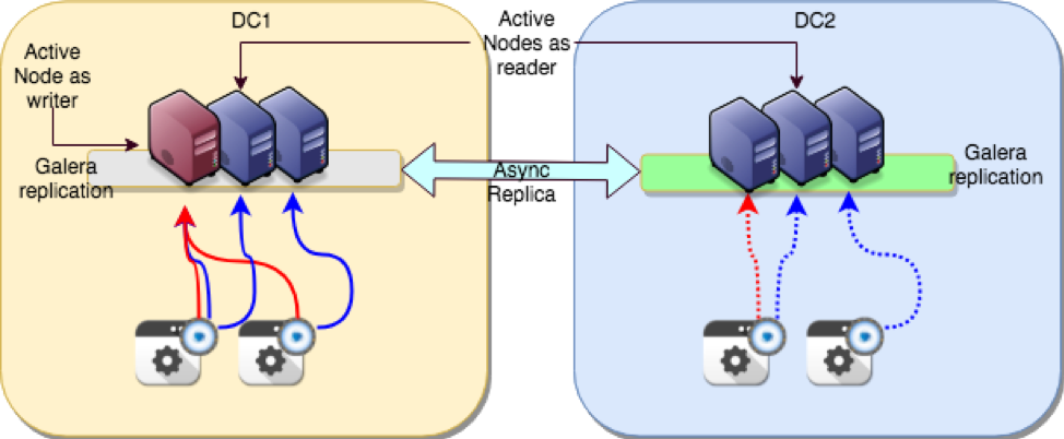
The right solution is easier than the wrong one, and there are already tools in place to make it work efficiently. Say you need to define your HA solution between the East and West Coast, or between Paris and Frankfurt. First of all, identify the real capacity of your network in each DC.
Then build a tightly coupled database cluster in location A and another tightly coupled database cluster in the other location B. Then link them using ASYNCHRONOUS replication.
Finally, use a tool like Replication Manager for Percona XtraDB Cluster to automatically manage asynchronous replication failover between nodes.
On top of all of that use a tool like ProxySQL to manage the application requests.
The full architecture is described here. 

Conclusions

The myth of using ANY solution based on tightly coupled database cluster on distributed geographic locations is just that: a myth. It is conceptually wrong and practically dangerous.

It MIGHT work when you set it up, it MIGHT work when you test it, it MIGHT even work for some time in production.

  By definition, it will break, and it will break when it is least convenient. It will break in an unpredictable moment, but because of a predictable reason.

You did the wrong thing by following a myth. Whenever you need to distribute your data over different geographic locations, and you cannot rely on a single physical channel (fiber) to connect the two locations, use asynchronous replication, period!

References

https://github.com/y-trudeau/Mysql-tools/tree/master/PXC
http://www.tusacentral.net/joomla/index.php/mysql-blogs/164-effective-way-to-check-the-network-connection-when-in-need-of-a-geographic-distribution-replication-.html
https://www.percona.com/blog/2013/05/14/is-synchronous-replication-right-for-your-app/

Sample test

#!/bin/bash 
test_log=/tmp/results_$(date +'%Y-%m-%d_%H_%M_%S').txt
exec 9>>"$test_log"
exec 2>&9
exec 1>&9
echo "$(date +'%Y-%m-%d_%H_%M_%S')" >&9

for ip in 11 12 13; do
  echo "  ==== Processing server 10.0.0.$ip === " 

  for size in 1 48 512 1024 4096;do
    echo " --- PING ---"
    ping -M do -c 5  10.0.0.$ip -s $size
    echo "  ---- Record Size $size ---- " 
    netperf -H 10.0.0.$ip -4 -p 3307 -I 95,10 -i 3,3 -j -a 4096 -A 4096  -P 1 -v 2 -l 20 -t TCP_RR -- -b 5 -r ${size}K,48K -s 1M -S 1M
    echo "  ---- ================= ---- ";
  done
   echo "  ==== ----------------- === ";
done